Temporal Context in Deep Nets for MLB Pitch Modeling: A Study of Lag Length and Architecture
Henry Wang
Final project for 6.7960, MIT
Outline

Introduction

Background

Methods

Results

Discussion

Introduction

*A very basic understanding of baseball is helpful, but not critical, for this blog. For an intro, see Baseball For Dummies Cheat Sheet.

We use pitch data from 5 years of Major League Baseball (MLB) games as a domain for assessing the behavior of deep learning methods on a real-world prediction task where empirical research has been limited. We explore how different inductive biases, feature representations, and evaluation methods behave in an autoregressive pitch modeling setting, using baseball as a novel test setting. We train and evaluate models on over 5 years of Statcast data from MLB games (2021-2025), predicting continuous pitch outcomes in terms of run expectancy changes. Our results yield interesting insights about the inductive biases of MLPs and LSTMs in the pitch modeling setting, highlighting risks in naively growing the input dimension without careful regularization.

Background & Related Work

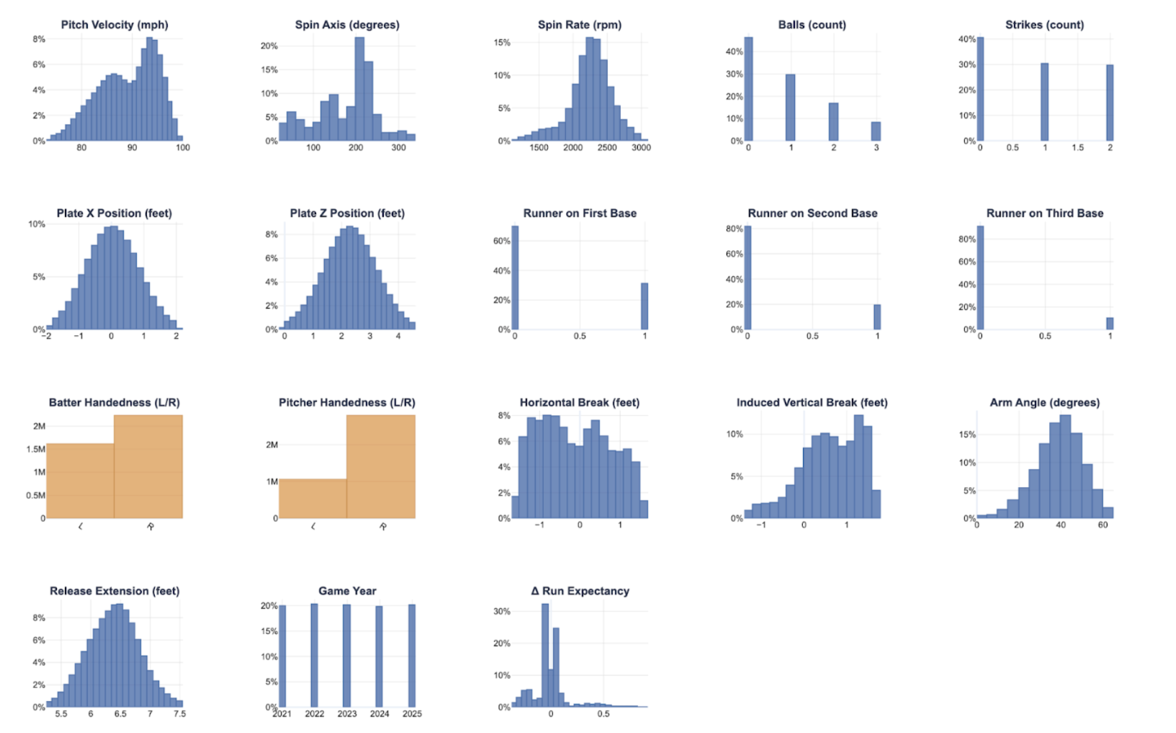
Sabermetrics, or baseball analytics, is the practice of applying scientific and mathematical principles to the game of baseball. This field, popularized by the film Moneyball, has become a mainstram practice in the sport. Every year, over 700,000 pitches are thrown in Major League Baseball (MLB), each being meticulously tracked by a wide array of technologies. Various optical and radar-based tracking systems allow analysts to build quantitative models using characteristics such as velocity, spin rate, and magnus-induced movement to characterize what makes pitches successful (by preventing runs).

The science of pitch modeling, in particular, has become a mainstream practice in the sabermetrics community. The goal of pitch modeling is to use information of pitches (release speed, trajectory, spin, etc.) to predict a run value, where allowing less runs is favorable for the pitcher. Existing work in this space has revealed key insights that inform player development and evaluation strategies used today. For example, pitch models (oftentimes referred to as Stuff+ models) suggest that higher velocity on fastballs predict better outcomes for the pitcher, which has transformed the way pitchers train and develop.

Run Expectancy
Pitch modeling, in its simplest form, treats each pitch as a regression problem with a continuous target (a run-based value) and a set of pitch characteristics as inputs, such as velocity, spin rate, and so forth [5, 6]. To understand the concept of run values, it is useful to think of a baseball game as a Markov chain, where states are combinations of baserunner configurations (are there runners on 1st, 2nd, and/or 3rd) and the number of outs (0, 1, or 2). There are \(2^3 = 8\) possible baserunner states and 3 possible out states, resulting in \(8 \times 3 = 24\) base–out states. The expected number of runs scored from a given base–out state to the end of the inning is called the run expectancy.

Run Expectancy Matrix
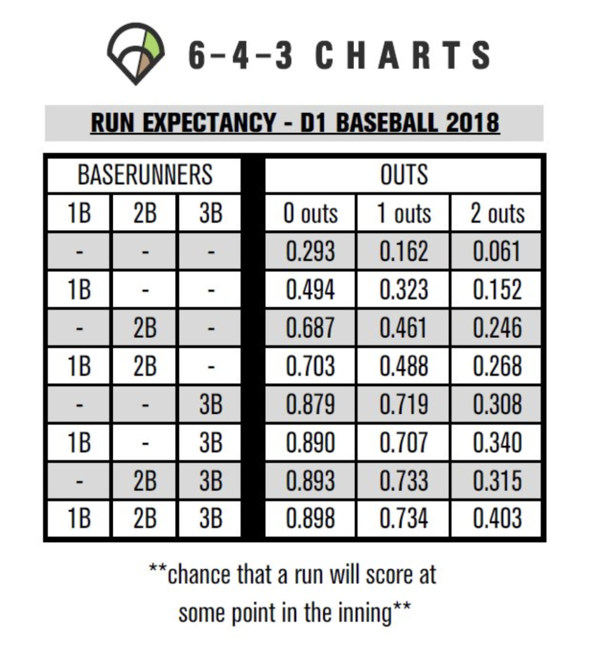
Figure 1. Example Run Expectancy Matrix for D1 Baseball 2018. The table shows the expected number of runs that will score from each base-out state to the end of the inning. Source: 6-4-3 Charts

Run expectancy can be defined more granularly using base–out–count states: this is the same idea as base–out states, except now we also condition on the ball–strike count. In full, there are 12 possible ball–strike counts, yielding \(24 \times 12 = 288\) base–out–count states.

Every pitch moves the game from one base–out–count state to another, each with its own run expectancy. The pitcher's goal is to reduce the overall run expectancy. The target we use is delta run expectancy (\(\Delta RE\)), meaning the change in run expectancy from before to after the pitch. This provides a numerical representation of the pitch's effectiveness at preventing runs.

As Figure 1 shows, the expected number of runs varies dramatically depending on the game situation. The formula for delta run expectancy is:

\[ \Delta RE = RE_{\text{after}} - RE_{\text{before}} + \text{Runs Scored on the Pitch} \]

As a concrete example, consider the following scenario: A relief pitcher enters the game with the bases loaded and one out. They allow a sacrifice fly to score the runner from third, with the other two runners not advancing.

Pitch Modeling as an Autoregressive Task

Over the past several years, the sabermetric community has come to recognize that pitch modeling is in fact an autoregressive task. Autoregressiveness, however, is not implemented through inductive biases of selected models, but rather through engineering the input features to capture what is thought to be autoregressive structure. For example, studies of pitch sequencing and pitch tunneling show that the effectiveness of one pitch can depend on the pitches the hitter has already seen during the plate appearance. Sequencing refers to how the pitcher arranges different pitch types over time to set up the hitter, while tunneling refers to making different pitches look nearly identical for as long as possible out of the hand before they break in different directions [7]. For example, a high fastball that raises the hitter's eyeline likely makes the incoming low curveball more effective, especially if they tunnel together.

In practice, pitch models are typically implemented as gradient boosting trees, which are good at capturing nonlinearities and high-level interactions. In this setting, autoregressive structure is injected by simply adding lagged features as inputs to the model. These can be raw lagged features (e.g., the velocity of the last pitch to see how much velo the pitcher added or "killed") or handcrafted ones (with measures of pitch tunneling being a prominent example). Despite some public research on sequence models for predicting pitch types [8], there is relatively little work exploring deep sequence models for run expectancies. Additionally, the pitch modeling setting is a relatively unexplored domain for empirical research in deep learning, despite the richness of data and clear underlying objectives.

Outside of baseball, there is a large literature on deep learning for time-series forecasting across domains such as finance, transportation, and climate, and surveys find that sequence models are oftentimes the superior model class for these tasks [9, 10]. However, this is not a guarantee, and previous research has shown that even simple temporal convolutional networks can beat LSTMs on standard sequence benchmarks and exhibit longer effective memory than vanilla recurrent networks [11]. This work is similar to studies that compare LSTMs to traditional time-series models (ARIMAs) under noisy economic or financial data [12]. However, beyond simply comparing predictive performance, we investigate how relative performance changes with different information budgets and examine the source of performance gaps. This project uses pitch modeling as a setting for understanding when sequence models offer advantages over traditional MLPs. I would argue this is a particularly interesting setting due to the notoriously random nature of baseball outcomes at the pitch level.

Research Questions

This project aims to address the following research objectives:

1. Effective memory and context usage in LSTMs vs "just add lags"
For a given lag length \(k\), how does the LSTM's advantage over the MLP evolve with pitch number within a plate appearance, if at all?

2. Inductive biases under noisy supervision
What do numerical results reveal about the differences in inductive biases of MLPs vs LSTMs in highly noisy, partially autoregressive environments?

We evaluate models using RMSE at both the pitch level (individual predictions) and pitcher level (aggregated by pitcher). The pitcher-level view is particularly relevant for player evaluation over a larger number of pitches (e.g. a season's worth of innings pitched).

Methods

Data
Pitch-level data from MLB Statcast was queried using the pybaseball Python package [13] for all seasons between 2021 and 2025, yielding a total of 3,833,701 pitches.

For every pitch, we have the relevant contextual and kinematic features characterizing the event. Table 1 provides the complete feature set used in this study:

Table 1. Feature Descriptions and Variable Types
Feature Variable Type Plain-English Definition
Pitch Velocity (mph) Kinematic Speed of the pitch as it leaves the pitcher's hand. Generally, higher fastball velocity and the ability to "kill" velocity on offspeed pitches is better for the pitcher.
Spin Axis (degrees) Kinematic Direction the ball is rotating around as it travels toward the plate, directly determining the direction of the spin-induced movement (Magnus force)
Spin Rate (rpm) Kinematic How fast the ball is spinning around its axis, directly determining the magnitude of the spin-induced movement (Magnus force).
Plate X Position (ft) Kinematic Horizontal location where the pitch crosses the front of home plate (inside/outside).
Plate Z Position (ft) Kinematic Height of the pitch above the ground as it crosses the front of home plate.
Horizontal Break (ft) Kinematic Side-to-side movement of the pitch caused by the Magnus force and seam-shifted wake.
Induced Vertical Break (ft) Kinematic Extra rise or drop on the pitch due to spin, beyond what gravity alone would do, caused by the Magnus force and seam-shifted wake.
Arm Angle (degrees) Kinematic The angle of the pitcher's arm at release (over-the-top vs. sidearm, etc.).
Release Extension (ft) Kinematic How far in front of the rubber the pitcher releases the ball. Higher extension means the ball is released closer to home plate, typically better for the pitcher.
Balls (count) Contextual Number of balls in the count before the pitch.
Strikes (count) Contextual Number of strikes in the count before the pitch.
Runner on First Base Contextual Indicator of whether there is a runner on first base.
Runner on Second Base Contextual Indicator of whether there is a runner on second base.
Runner on Third Base Contextual Indicator of whether there is a runner on third base.
Batter Handedness (R/L) Contextual Whether the batter is hitting left-handed or right-handed. Typically, being the opposite handedness as the pitcher favors the batter.
Pitcher Handedness (R/L) Contextual Whether the pitcher throws left-handed or right-handed. Typically, being the same handedness as the batter favors the pitcher.
Game Year Contextual Season year in which the pitch was thrown. Accounts for the yearly variation in run scoring environment.
Delta Run Expectancy Target variable Change in expected runs for the inning from before to after the pitch (the pitch's run value).

Feature Distributions
Figure 2. Feature Distributions of 3.8 Million Pitches from MLB Statcast (2021-2025). Histograms show the distribution of kinematic and contextual features across all pitches. Yellow bars indicate categorical features.

Data were split into train/validation/test (80/10/10) in a pitcher-stratified fashion to avoid pitcher-specific leakage. The random seed was fixed to eliminate confounding variables when comparing model performance.

Autoregressive Features
We introduce autoregressive structure by adding lagged features for kinematic features: velocity, spin axis, spin rate, arm angle, release extension, and plate location (horizontal and vertical). Together, they summarize the "look" and movement of prior pitches to the hitter, the primary aspect of pitch sequencing. We exclude contextual features, as the autoregressive bias for these features is likely minimal. We define a time series at the plate-appearance (PA) level. Thus, a PA where the hitter saw 5 pitches corresponds to a length-5 sequence, and the 5th pitch in that PA has \(k = 4\) lags of features available.

MLPs
We build and train several fixed-architecture residual MLPs to predict delta run expectancy on the aforementioned features, varying the number of lagged features available in the input representation, growing the input dimension linearly with \(k\). We one-hot encode categorical features and impute missing values with a sentinel. We Z-score features for standardization and then train the MLP (input layer → four residual ReLU blocks → linear output) with Adam (\(\text{lr} = 10^{-3}\), weight decay \(\lambda = 10^{-5}\)), MSE loss, gradient clipping, and early stopping on validation MSE. We forgo hyperparameter tuning for this work, given the time and compute constraints of the semester.

LSTMs
In the sequence modeling setting, we model each pitch as the last step of a short sequence and let an LSTM learn how recent pitches shape the outcome. For a given history length \(k\), the input is ordered as \([x_{t-k}, \ldots, x_{t-1}, x_t]\), where earlier steps contain lagged deltas of kinematic and location features and the final step also holds the current pitch's one‑hot–encoded context (count, handedness, runners, etc.). We apply the same imputation and scaling process used for MLPs. A two‑layer LSTM (hidden dimension \(h = 128\), mild dropout) feeds a ReLU head and a linear output that predicts the change in run expectancy. We optimize with Adam (\(\text{lr} = 10^{-3}\), weight decay \(\lambda = 10^{-5}\)), use gradient clipping, and early stopping on validation MSE, consistent with the MLPs. All models use the same optimization strategy and early stopping criteria to ensure an equal comparison.

Evaluation Metrics

We use two modes of evaluation: at the pitch-level RMSE and at the pitcher-level RMSE. Baseball outcomes are inherently noisy, and even very strong models typically achieve modest performance in this setting. Our focus is therefore on relative performance across model classes instead of absolute magnitudes. The pitcher-level view is useful for player evaluation, capturing how well each model differentiates between pitchers over many pitches. Pitcher-level RMSE provides insight into how well models can distinguish between different pitchers' abilities in the aggregate.

Results

We find strong evidence that LSTMs outperform MLPs on both pitch-level RMSE and pitcher-level RMSE in the autoregressive setting, which is not entirely surprising. The interesting finding here is that the performance gap increases with the number of lags and is driven by worsening MLP performance rather than improvements in the LSTM (Figures 3 and 4). Linearly increasing the number of lagged features fed to the fixed-architecture MLP appears to negatively impact the signal-to-noise ratio, hindering results in both training and out-of-sample contexts. By contrast, the LSTM gains little from additional lags but does not deteriorate, consistent with an ability to down-weight or forget noisy history. The LSTM provides consistent improvements ranging from approximately 1-3% in RMSE across different lag values (Figure 4). Ultimately, these results suggest that when we care about longer pitch histories, sequence models like LSTMs are a safer default than simply adding more lags to an MLP, though a larger or more strongly regularized MLP might narrow this gap.

Predictive Performance: LSTM vs MLP
Figure 3. Predictive Performance: LSTM vs MLP (Same Information Budget). RMSE comparison across different lag lengths for both pitch-level (left) and pitcher-level (right) evaluation. Shaded regions show ±1 standard deviation. The LSTM (green) maintains consistent performance while the MLP (purple) degrades as more lagged features are added.

LSTM Improvement over MLP (%)
Figure 4. LSTM Improvement over MLP (%). Percentage RMSE improvement of LSTM over MLP across different lag lengths. Error bars show ±1 standard deviation. Left panel shows pitch-level improvement; right panel shows pitcher-level improvement. The LSTM advantage peaks at lag 2 with 3.13% improvement at pitch-level and 3.11% at pitcher-level.

Performance by Pitch Number
As a next step, we break performance down by the pitch's position within the plate appearance (up to the 8th pitch) for a few lagged models (\(k \in \{3, 5, 7\}\)). For each \(k\), the LSTM's advantage over the MLP grows nearly monotonically as more pitches are seen, peaks around pitch \(k\), and then starts to taper off (Figure 5). This pattern fits the intuition that the LSTM gains most once it has access to its full \(k\)-pitch history, with additional context providing diminishing returns. Later pitch numbers are also rarer in the data, so the bars at 7 and 8 should be interpreted with a bit more caution.

LSTM Advantage by Pitch Number
Figure 5. LSTM Advantage by Pitch Number. Percentage RMSE improvement of LSTM over MLP at different pitch numbers within the plate appearance, shown for lag values \(k \in \{3, 5, 7\}\). Top row shows pitch-level RMSE; bottom row shows pitcher-level RMSE. The LSTM advantage peaks around pitch \(k\) (the lag length), then diminishes.

Figures 3 and 4 show LSTM stability and percentage improvement across lags, while Figure 5 reveals how LSTM advantage varies within each plate appearance.

Discussion & Conclusions

Our results yield several interesting lessons about how strengths of inductive biases of deep learning models manifest in the pitch modeling setting. First, we see strong evidence of limitations in the "just add lags" strategy for MLPs. We find that as the number of lags increases, a fixed capacity residual MLP eventually breaks down, even though the model technically has more information. This suggests that, in noisy autoregressive environments such as baseball, naively growing the input dimension may harm the signal-to-noise ratio and hurt the ability to learn useful models, especially when capacity and regularization are not adjusted accordingly.

Second, under the same information budget, the LSTM is more robust to additional context, but in an interesting fashion. Its performance advantage grows as we add lags, but is driven almost entirely by the MLP getting worse, not by the LSTM getting better. When we break results down by pitch number within the plate appearance, the LSTM's advantage grows as the sequence unfolds, peaks once it has roughly \(k\) pitches of usable history, and then drops off. This is consistent with an effective memory window, as the recurrent architecture likely learns to discard older, noisy context rather than overfitting to it. However, the LSTM will fail to generalize well to sequences beyond its information budget, at times catastrophically, highlighting a need to carefully tailor sequence length to the data at hand.

Taken together, these findings highlight that architecture choice matters even in relatively simple autoregressive problems with short horizons. In this pitch modeling setting where label noise is substantial but autoregressive signal is likely present, stacking lagged features into feed-forward models fail due to the weak temporal biases baked into MLPs. The results suggest that models with temporal structure (LSTMs) are a safer default once we start to care about even modest history lengths due to their ability to "forget" about noisy histories. These insights may generalize to other noisy autoregressive prediction tasks beyond baseball.

Limitations

This work has several limitations. We only compare a single family of MLPs and a single LSTM configuration, without extensive hyperparameter tuning or architectural search, due to the compute available as well as the semester's time constraints. All results are specific to one domain (MLB pitch data) and one target (delta run expectancy). As such, our conclusions should be viewed as empirical case studies of inductive bias rather than definitive verdicts about architecture choice. Future work could explore more architectures and hyperparameter configurations to validate these findings.

References

[1] Major League Baseball (2021-2025). Statcast data. Baseball Savant. Retrieved from https://baseballsavant.mlb.com/

[2] Paszke, A., Gross, S., Massa, F., Lerer, A., Bradbury, J., Chanan, G., ... & Chintala, S. (2019). PyTorch: An imperative style, high-performance deep learning library. Advances in Neural Information Processing Systems, 32.

[3] Hochreiter, S., & Schmidhuber, J. (1997). Long short-term memory. Neural Computation, 9(8), 1735-1780.

[4] Wang, H. (2024). Temporal Context in Deep Neural Networks for MLB Pitch Prediction. Final project for MIT 6.7960: Deep Learning (Fall 2024).

[5] Asel, J. (2021). Rethinking the True Run Value of a Pitch With a Pitch Model. Driveline Baseball. Retrieved from https://www.drivelinebaseball.com/2021/09/rethinking-the-true-run-value-of-a-pitch-with-a-pitch-model/

[6] Weinberg, B. Predicting Run Production and Run Prevention in Baseball: The Impact of Sabermetrics. Retrieved from ResearchGate

[7] Prospectus Feature: Updating Pitch Tunnels. Baseball Prospectus. Retrieved from https://www.baseballprospectus.com/news/article/37436/prospectus-feature-updating-pitch-tunnels/

[8] No Pitch is an Island: Pitch Prediction with Sequence-to-Sequence Deep Learning. FanGraphs Community Research. Retrieved from https://community.fangraphs.com/no-pitch-is-an-island-pitch-prediction-with-sequence-to-sequence-deep-learning/

[9] Kong, X., Chen, Z., Liu, W., Ning, K., Zhang, L., Marier, S. M., ... & Xia, F. (2025). Deep learning for time series forecasting: a survey. International Journal of Machine Learning and Cybernetics, 16, 5079-5112.

[10] Deep learning for time series forecasting: a survey. Retrieved from ResearchGate

[11] Bai, S., Kolter, J. Z., & Koltun, V. (2018). An empirical evaluation of generic convolutional and recurrent networks for sequence modeling. arXiv preprint arXiv:1803.01271.

[12] Siami-Namini, S., & Namin, A. S. (2018). Forecasting economics and financial time series: ARIMA vs. LSTM. arXiv preprint arXiv:1803.06386.

[13] LeDoux, J., & Schorr, M. (2024). pybaseball: A Python package for baseball data retrieval and analysis. GitHub repository. Retrieved from https://github.com/jldbc/pybaseball